


 This question comes up from time to time in our Microsoft Excel workshops. VLOOKUP is one of the very helpful functions in Microsoft Excel. It allows us to lookup values from various lists and use the results as necessary.
For insatnce, I might have the following list:
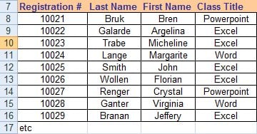
And if I would like to find the Class Title that corresponds to Registration Number 10024, I can use VLOOKUP as follows:
=VLOOKUP(10024,A7:D16,4,FALSE)
In this case, VLOOKUP tries to find an exact match for 10024 and if it finds it, it returns the Class Title. In this case, it would return Word.
But what if VLOOKUP doesn't find the desired results. For instance if I am try to look for Registration 12020 (which doesn't exist in the list), then VLOOKUP would return: #N/A
While this may not be a big deal in some situations, it can be quite distracting if I am using VLOOKUP to populate a column in a report from another table (which is what VLOOKUP is best at). Suddenly my report may have several of these #N/A's which ideally would be replaced by something more user friends or be suppressed all together.
How can you manage or suppress the #N/A?
To manage or suppress the #N/A's, you need to make use of 2 functions:
- ISNA() which determines if the result of the VLOOKUP is #N/A
- IF() which allows you to replace the #N/A result or suppress it
This is the syntax of the "smarter" VLOOKUP statement:
=IF(ISNA(VLOOKUP(12020,A7:D16,4,FALSE)),"Not Found",VLOOKUP(12020,A7:D16,4,FALSE))
Or if you want to suppress it all together:
=IF(ISNA(VLOOKUP(12020,A7:D16,4,FALSE)),"",VLOOKUP(12020,A7:D16,4,FALSE))