<img height="1" width="1" style="display:none" src="https://www.facebook.com/tr?id=289291844809425&amp;ev=PageView&amp;noscript=1">
Less Is More Blog Productivity Tips

Join us at the Webinars

2021_Webinars_Schedule_People-OnTheGo

Click for our Webinars Schedule.

The Perfect 15-Minute Day Method is here!

Promotiona_Video_Thumbnail_Rev2.jpg

Order the book, eBook, journal, or eCourse to get started right away and inject a healthy dose of accomplishments and happiness in your workday and beyond!

Learn more!

Get Our Free eBook

The Results Curve: How to Manage Focused and Collaborative Time

Less-Is-More Blog by Pierre Khawand

Accomplishing More With Excel: Sorting Excel PivotTable Reports using columns instead of grand totals

Posted by Pierre Khawand on Mon, May 24, 2010 @ 08:39 AM

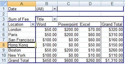
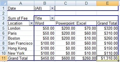
When you are working with a PivotTable report, you can easily sort the report manually or alphabetically in ascending or descending order, but you can also sort it by ascending and desending order of the grand total as shown in the report below: 

PivotTable Sort Grand Total

But how about if you want to sort the report by the PowerPoint instead of the grand total?

There is a way:

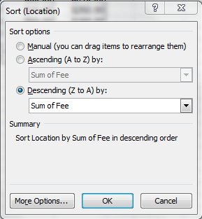
First: Right-mouse click on any of the location field (or any of the location items such as San Francisco for instance) and then from the popup menu, select the "Sort" menu item, and then the "More Sort Options…" sub-menu item. The Sort (Location) window opens up. 

Second: Click the "Descending" option and select "Sum of Fee" from the dropdown box:

PivotTable Reports Sort Options

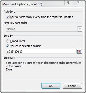
Third: Click the "More Options" button. The More Sort Options (Location) window opens up. Click the "Values in selected column" option and then enter the desired range (in this case if we want to sort by the values in the Excel column, this would be $D$5:$D$10):

More options in Excel PivotTables

Voila! Here is the resulting report

Excel PivotTable Reports sorted by column
 

Additional Resources


Topics: Microsoft Office 2007, Microsoft Excel Tutorial

Question & Answer: How do I set a password to protect my Microsoft Excel Workbook?

Posted by Pierre Khawand on Sun, May 02, 2010 @ 05:55 PM

If you would like to password protect an Excel workbook, the process is easy and it is the same process by which you can also protect other Microsoft Office documents such as Microsoft Word and Microsoft PowerPoint. The steps below demonstrate how to assign a password for opening and for modifying an Excel workbook.

Please note while the steps below illustrate the process in Microsoft Excel 2007, the steps are pretty much the same in Microsoft Excel 2003 and even Microsoft Excel 2010. 

First: After you save your document, use the Save As option from the Office Button menu to open the Save As window.

Excel 2007 Password Protect

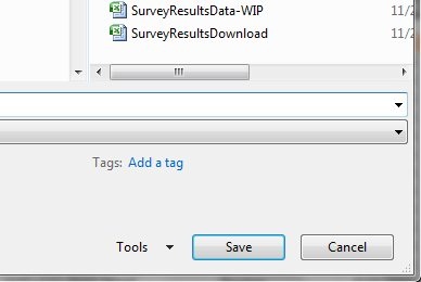
Second: In the Save As window, click on the drop down arrow next to the Tools button that is near the Save and Cancel buttons as illustrated below.

Excel 2007 Password Protect

Third:  Then from the list of options, select the General Option to get the General Options window:

Excel 2007 Password Protect

You can provide two different passwords, one for opening the document, and one for modifying the document. This allows you to provide certain people the ability to view the document but not edit it, while allowing only designated people to edit the document.

You will then be prompted to confirm the passwords you have entered, and then once you confirm, and save the document, you will also be prompted to confirm that you want to replace the existing document, in which case you want to click Yes to confirm.

One word of caution though: "keep the password in a safe place."

Additional Resources

The Microsoft Excel Techniques workshop (see upcoming Webinar on May 11, 2010)

Topics: Microsoft Office 2007, Microsoft Excel Tutorial

Question and Answer: How do I suppress the #N/A results when using VLOOKUP in Microsoft Excel?

Posted by Pierre Khawand on Wed, Mar 17, 2010 @ 09:01 AM

Microsoft Excel VLOOKUP Suppressing #N/AThis question comes up from time to time in our Microsoft Excel workshops. VLOOKUP is one of the very helpful functions in Microsoft Excel. It allows us to lookup values from various lists and use the results as necessary.

For insatnce, I might have the following list:
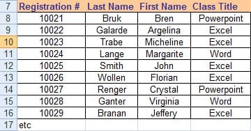
 

Microsoft Excel VLOOKUP

And if I would like to find the Class Title that corresponds to Registration Number 10024, I can use VLOOKUP as follows:

=VLOOKUP(10024,A7:D16,4,FALSE)

In this case, VLOOKUP tries to find an exact match for 10024 and if it finds it, it returns the Class Title. In this case, it would return Word.

But what if VLOOKUP doesn't find the desired results. For instance if I am try to look for Registration 12020 (which doesn't exist in the list), then VLOOKUP would return: #N/A

While this may not be a big deal in some situations, it can be quite distracting if I am using VLOOKUP to populate a column in a report from another table (which is what VLOOKUP is best at). Suddenly my report may have several of these #N/A's which ideally would be replaced by something more user friends or be suppressed all together.

How can you manage or suppress the #N/A?

To manage or suppress the #N/A's, you need to make use of 2 functions:

  • ISNA() which determines if the result of the VLOOKUP is #N/A
     
  • IF() which allows you to replace the #N/A result or suppress it

This is the syntax of the "smarter" VLOOKUP statement:

=IF(ISNA(VLOOKUP(12020,A7:D16,4,FALSE)),"Not Found",VLOOKUP(12020,A7:D16,4,FALSE))

Or if you want to suppress it all together:

=IF(ISNA(VLOOKUP(12020,A7:D16,4,FALSE)),"",VLOOKUP(12020,A7:D16,4,FALSE))

Additional Excel Resources

Microsoft Excel Techniques workshop

Advanced Excel PivotTables

Microsoft Excel Macros
Topics: Microsoft Office 2007, Microsoft Excel Tutorial